線性回帰分析(Linear regression)
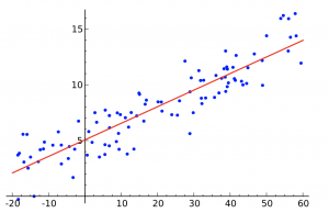
Linear regression is a linear model, e.g. a model that assumes a linear relationship between the input variables (x) and the single output variable (y). More specifically, that output variable (y) can be calculated from a linear combination of the input variables (x).
Features (variables)
Each training example consists of features (variables) that describe this example (i.e. number of rooms, the square of the apartment etc.)

n – number of features
Rn+1 – vector of n+1 real numbers
Parameters
Parameters of the hypothesis we want our algorithm to learn in order to be able to do predictions (i.e. predict the price of the apartment).

Hypothesis
The equation that gets features and parameters as an input and predicts the value as an output (i.e. predict the price of the apartment based on its size and number of rooms).

For convenience of notation, define X0 = 1
Cost Function
Function that shows how accurate the predictions of the hypothesis are with current set of parameters.

xi – input (features) of ith training example
yi – output of ith training example
m – number of training examples
Batch Gradient Descent
Gradient descent is an iterative optimization algorithm for finding the minimum of a cost function described above. To find a local minimum of a function using gradient descent, one takes steps proportional to the negative of the gradient (or approximate gradient) of the function at the current point.
We need to simultaneously update  for j = 0, 1, …, n


 – the learning rate, the constant that defines the size of the gradient descent step
 – jth feature value of the ith training example
 – input (features) of ith training example
yi – output of ith training example
m – number of training examples
n – number of features
Feature Scaling
To make linear regression and gradient descent algorithm work correctly we need to make sure that features are on a similar scale.

For example “apartment size” feature (e.g. 120 m2) is much bigger than the “number of rooms” feature (e.g. 2).
In order to scale the features we need to do mean normalization

– jth feature value of the ith training example
 – average value of jth feature in training set
 – the range (max – min) of jth feature in training set.
Regularization
Overfitting Problem
If we have too many features, the learned hypothesis may fit the training set very well:

Solution to Overfitting
Here are couple of options that may be addressed:
- Reduce the number of features
- Manually select which features to keep
- Model selection algorithm
- Regularization
- Keep all the features, but reduce magnitude/values of model parameters (thetas).
- Works well when we have a lot of features, each of which contributes a bit to predicting y.
Regularization works by adding regularization parameter to the cost function:

※Note that you should not regularize the parameter 
 – regularization parameter
In this case the gradient descent formula will look like the following:

from: